When it comes to machine learning, some algorithms ask for more than they give. They demand heavy tuning, heaps of training data, and even then, they tend to overthink everything. Naive Bayes doesn’t bother with any of that. It offers quick results, handles classification tasks well, and doesn’t need a lot of babysitting. Whether you're building a basic text analyzer or categorizing customer feedback, this algorithm finds its place with ease.

But how can something so basic manage to deliver such consistent performance? Let’s break it down.

What Naive Bayes Really Means

At first glance, Naive Bayes sounds like a contradiction: it’s both naïve and based on Bayes’ Theorem, which is anything but naive. The key here is the assumption the algorithm makes—it treats every feature as independent from the others, given the outcome. That’s the "naive" part. In real life, that assumption is often incorrect, yet the model still manages to hold its ground in practical use.

The Math in Plain English

You start with Bayes' Theorem:

P(A∣B)=P(B∣A)⋅P(A)P(B)P(A|B) = \frac{P(B|A) \cdot P(A)}{P(B)}P(A∣B)=P(B)P(B∣A)⋅P(A)​

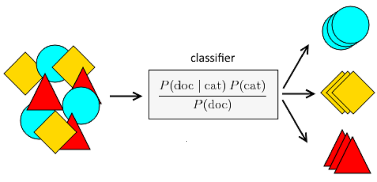
Translated: the probability of a class (A) given the input features (B) depends on how likely those features are in that class, multiplied by how common that class is overall, divided by how common the features are across all examples.

Now here’s where it gets clever: instead of considering every possible interaction between features—which becomes impractical very quickly—Naive Bayes just assumes independence and multiplies their probabilities individually.

This shortcut helps the model stay lightweight and quick, even on datasets with thousands of features.

Common Variants and Where They Work Best

Not all Naive Bayes models follow the same logic. The framework has a few core versions, each tailored for different types of data. Understanding these helps match the right model to the problem at hand.

1. Gaussian Naive Bayes

This version assumes your features follow a normal distribution. It's a natural fit when your input variables are continuous, like weight, height, or temperature. For instance, in medical prediction models where inputs are numeric, Gaussian Naive Bayes tends to perform reliably without much transformation.

2. Multinomial Naive Bayes

If your data involves counting—say, how often a term appears in a document—this variant is what you want. It's widely used in natural language processing, where frequency is a key consideration. Applications like document categorization or language detection benefit from this model due to its focus on term occurrence.

3. Bernoulli Naive Bayes

Instead of tracking how many times something appears, Bernoulli Naive Bayes asks whether it shows up at all. It deals in binary values, focusing on presence or absence. This is useful when frequency becomes irrelevant and even a single occurrence can shift the outcome.

How to Build a Naive Bayes Model (Step-by-Step)

If you’re looking to create your first Naive Bayes model, you won’t need much more than a standard dataset and a few lines of Python. The learning curve is shallow, making it perfect for straightforward classification tasks.

Step 1: Prepare Your Data

Start with your inputs (features) and their corresponding labels (categories). For text data, begin with preprocessing: lowercasing, removing punctuation, tokenizing, and converting the results into a numerical format.

python

CopyEdit

from sklearn.model_selection import train_test_split

# Splitting the dataset into training and testing sets

X_train, X_test, y_train, y_test = train_test_split(features, labels, test_size=0.3)

Step 2: Choose the Right Model

Select the Naive Bayes version based on your data type:

python

CopyEdit

from sklearn.naive_bayes import MultinomialNB, GaussianNB, BernoulliNB

model = MultinomialNB() # You can also use GaussianNB or BernoulliNB as needed

Step 3: Train the Model

Fit the model to your training data. This step helps the algorithm estimate the probabilities it needs for classification.

python

CopyEdit

model.fit(X_train, y_train)

Step 4: Make Predictions

Now use the trained model to predict outcomes for the test data.

python

CopyEdit

predictions = model.predict(X_test)

Step 5: Evaluate the Results

Finally, check how well your model did. Accuracy, precision, and recall are useful metrics here.

python

CopyEdit

from sklearn.metrics import accuracy_score

print("Accuracy:", accuracy_score(y_test, predictions))

That’s all it takes to get a working model. The overall workflow is refreshingly straightforward, and you don’t need dozens of parameters to tune.

Known Limitations

Of course, no algorithm is flawless. One limitation of Naive Bayes comes from its strong independence assumption. In real-world datasets, features often influence each other. For instance, in customer behavior data, purchasing one item might be closely linked to buying another. Naive Bayes overlooks such connections, which can sometimes lead to less accurate predictions.

Another common issue is the zero-frequency problem. If the training data never contained a certain value or word, the algorithm assigns a zero probability to any prediction involving it. That’s a problem because it wipes out the entire calculation.

The usual fix is Laplace smoothing, which adds a small number (like 1) to every count to avoid zeros.

python

CopyEdit

model = MultinomialNB(alpha=1.0) # Applies Laplace smoothing

It’s a small adjustment, but it helps the algorithm stay functional even when new or rare features appear in test data.

Final Thoughts

Naive Bayes isn’t the flashiest tool in machine learning, but it’s one of the most practical. It doesn’t require endless tweaking, it trains in seconds, and it performs dependably in a wide range of scenarios. Whether you're building a filter for product reviews or organizing messages by topic, it’s a model that gets the job done without overcomplicating the process.

It's not designed to handle every case, especially those involving intricate relationships between inputs. But for clear-cut classification tasks—especially when working with text or small datasets—it brings results quickly and cleanly. If you're starting and want a dependable tool that's easy to interpret and even easier to implement, this one earns a spot near the top of your shortlist.